CALCULATION OF MS SIGNALS:
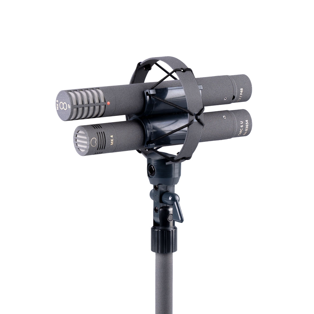
Two microphones are used: the microphone for the mid channel M is directed forwards, while the Fig-8 microphone for the side channel S is directed with its positive lobe at -90 °.
After the general microphone equation, the two microphones can be described as follows:
M = (1-a) + a * cos (β);
S = cos (β + 90 °); where a = ball portion; β = angle of incidence;
The level at β = 0 ° is 1;
The decoding of the two signals is performed by sum and difference, wherein the proportion of Fig-8 can be set arbitrarily. The factor k (level of the S signal) determines the resulting stereo width.
L = M + k * S;
R = M - k * S; where k = level of S;
After inserting the above microphone equations into these decoding rules and some transformation operations:
L = (1-m) + m * cos (β + θ);
R = (1-m) + m * cos (β-θ); where m = omni portion; β = angle of incidence;
The resulting signals L and R thus correspond to first order microphones in a coincident arrangement, which are arranged at an angle ± θ to one another, ie at an offset angle of 2θ.
The angle θ results from θ = atan (k / a) -> the more S is mixed, the larger the opening angle.
The level p on the main axis of the virtual microphone is given by p = (1-a) + √ (k² + a²); -> the more S mixed, the greater the level.
The pressure gradient component m of the resulting virtual microphone results from m = √ (k² + a²) / p -> the more Fig-8 is mixed, the greater the pressure gradient component.
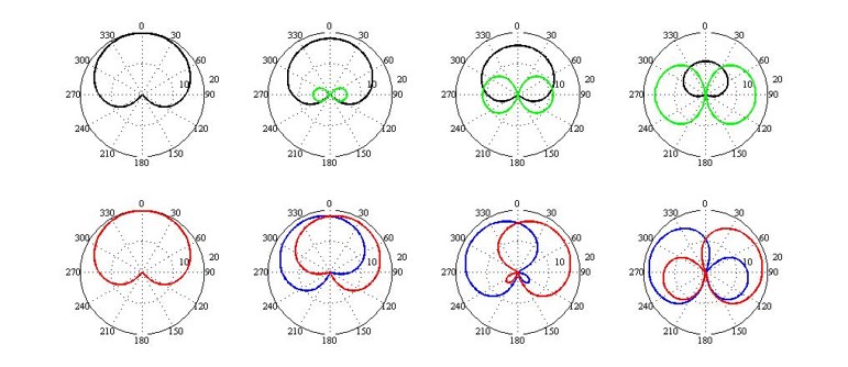
The following graphic illustrates the signals M and S (black and green), which become respectively L and R (blue and red), at different k values (levels of S):